Visualizing deep learning with galaxies, part 2
In the previous post, we examined the feature space of galaxy morphological features. Now, we will use the Grad-CAM algorithm to visualize the parts of a galaxy image that are most strongly associated with certain classifications. This will allows us to identify exactly which morphological features are correlated with low- and high-metallicity predictions.
- Galaxies, neural networks, and interpretability
- Binning the galaxies into metallicity classes
- A CNN classification model
- Explaining model predictions with Grad-CAM
- Conclusions
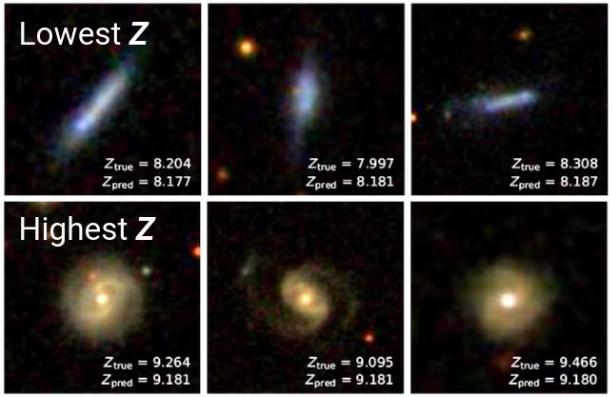
Up til this point, we have been interested in predicting a galaxy's elemental abundances from optical-wavelength imaging. Using the fast.ai library, we were able to train a deep CNN and estimate metallicity to incredibly low error in under 15 minutes. We then used dimensionality reduction techniques to help visualize the latent structure of CNN activations, and identified how morphological features of galaxies are associated with higher or lower metallicities.

In this post, we will look more closely at the CNN activation maps to see which parts of the galaxies are associated with predictions of low or high metallicity. This method of interpretation is sometimes referred to as image attribution. We investigate galaxy evolution using interpretable machine learning in my most recent paper.
One key difference between this analysis and the previous ones is that we will definine the CNN task as a binary classification problem rather than a regression problem. Once we have trained the classifier to distinguish low- and high-metallicity galaxies, we will be able to produce activation maps for both classes, even though the CNN will only predict one of the two. Setting up this classification task is no more difficult than the previous regression problem using the fastai DataBlock API.
fastai v2 library has been officially released, so definitely try it out if you haven’t yet! I’ve previously referred to this as the fastai2 library, but now it can be found in the main repository: https://github.com/fastai/fastai.
There's no obvious way to define metallicity "classes" since the distribution is unimodal and smooth. We can use pd.cut to sort low, medium, and high metallicities into bins $(8.1, 8.7]$, $(8.7, 9.1]$, and $(9.1, 9.3]$.
df['Z'] = pd.cut(
    df.metallicity,
    bins=[8.1, 8.7, 9.1, 9.3],
    labels=['low', 'medium', 'high']
)

df.Z.value_counts()
The majority are labeled as medium metallicites, but we will dropping things, such that our remaining data comprises two well-separated classes. The remaining low- and high-metallicity galaxies have slightly imbalanced classes, but this imbalance isn't be severe enough to cause any issues. (In more problematic cases, we could try resampling or weighting our DataLoaders, or weighting the cross entropy loss.)
df = df[df.Z != 'medium']

df.Z.value_counts()
DataBlocks for classification
Now that we have a smaller DataFrame with a column of metallicity categories (Z), we can construct the DataBlock. There are a few notable differences between this example and the previous DataBlock for regression:
- we use
CategoryBlockrather thanRegressionBlockas the second argument toblocks - we supply
ColReader('Z')forget_y - we have zoomed in on the images and only use the central 96×96 pixels, which will allow us to interpret the activation maps more easily
Afterwards, we populate ImageDataLoaders with data using from_dblock().
dblock = DataBlock(
    blocks=(ImageBlock, CategoryBlock),
    get_x=ColReader('objID', pref=f'{ROOT}/images/', suff='.jpg'),
    get_y=ColReader('Z'),
    splitter=RandomSplitter(0.2, seed=seed),
    item_tfms=[CropPad(96)],
    batch_tfms=aug_transforms(max_zoom=1., flip_vert=True, max_lighting=0., max_warp=0.) + [Normalize],
)

dls = ImageDataLoaders.from_dblock(dblock, df, path=ROOT, bs=64)
We can show a few galaxies to get a sense for what these high- and low-metallicity galaxies look like, keeping in mind that many "normal" spiral galaxies with typical metallicities have been excluded.
dls.show_batch(max_n=8, nrows=2)
Constructing a simple CNN
Next, we will construct our model. We will use the fast.ai ConvLayer class instead of writing out each sequence of 2d convolution, ReLU activation, and batch normalization layers. After the ConvLayers, we pool the activations, flatten them so that they are of shape (batch_size, 128), and pass them through a fully-connected (linear) layer.
model = nn.Sequential(
    ConvLayer(3, 32),
    ConvLayer(32, 64),
    ConvLayer(64, 128),
    nn.AdaptiveAvgPool2d(1),
    Flatten(),
    nn.Linear(128, dls.c)
)
That's it! We have a tiny 4-layer (not counting the pooling and flattening operations) neural network! Since there are only two classes, the DataLoaders knows that dls.c = 2 (even though there was a third class, galaxies with medium metallicities, but we've removed all of those examples from the catalog).
This final linear layer will output two floating point numbers. Although they might take on values outside the interval $[0, 1]$, they can be converted into probabilities by using the softmax function, and this is done implicitly as part of the nn.CrossEntropyLoss, which we will cover below.
Optimization and metrics
We can create a fast.ai Learner object just like before. Since we are working on a classification problem, the Learner assumes that we want a flattened version ofnn.CrossEntropyLoss. Thus, the argument to loss_func is optional (unlike in the previous the regression problem, where we needed to specify RMSE as the loss function). In this example, we do also have the option of passing in a weighted or label-smoothing cross entropy loss function, but it's not necessary here.
Cross entropy loss is great because it's the continuous, differentiable, negative log-likelihood of the class probabilities. On the flip side, it's not obvious how to interpret this loss function; we're more accustomed to seeing the model accuracy or some other metric. Fortunately, we can supply additional metrics to the Learner in order to monitor the model's performance. One obvious metric is the accuracy. We can also look at the area under curve of the receiving operator characteristic and the $F_1$ score (RocAuc and F1Score, respectively, in fast.ai). If we pass
metrics = [accuracy, RocAuc(), F1Score()]
to the Learner constructor, these metrics will be printed for the validation set after every epoch of training.
learn = Learner(
    dls,
    model,
    opt_func=ranger,
    metrics=[accuracy, RocAuc(), F1Score()]
)
Cool! Now let's pick a learning rate (LR) and get started. By the way, shallower models tend to work better with higher learning rates. So it shouldn't be a surprise that the LR finder identifies a higher LR than before (where we used a 34-layer xresnet).
learn.lr_find()
We can fit using the one-cycle (fit_one_cycle()) schedule as we did before. Here I've chosen 5 epochs just to keep it quick.
fit_flat_cos() scheduler works well for classification problems (and not regression problems). It might be worth a shot if you’re training a model from scratch — but if you’re using transfer learning, then I recommend sticking to fit_one_cycle(), since the "warmup phase" seems to be necessary for good results.
learn.fit_one_cycle(5, 8e-2)
In three minutes of training, we can achieve 95% in accuracy, ROC area-under-curve, and $F_1$ score. We can certainly do better (>98% for each of these metrics) if we trained for longer, used a deeper model, or leveraged transfer learning, but this performance is sufficient for revealing further insights. After all, we want to know which morphological features are responsible for the low- and high-metallicity predictions. Indeed, shallower neural networks with fewer pooling layers produce activation maps that are easier to interpret!
Finally, I would be remiss if I didn't mention that fast.ai offers a ClassificationInterpretation module! It can be used to plot a confusion matrix.
interp = ClassificationInterpretation.from_learner(learn)

interp.plot_confusion_matrix()
plt.xlabel(r'Predicted $Z$', fontsize=12)
plt.ylabel(r'True $Z$', fontsize=12);
ClassificationInterpretation can also plot the objects with highest losses, which is helpful for diagnosing what your model got wrong. Not only that, but it also has the Grad-CAM visualization baked in, so that you can visualize exactly which parts of the image it has gotten incorrect. But in the next section, we will implement Grad-CAM ourselves using Fastai forward and backwards hooks. If you're unfamiliar with this topic, it could be helpful to refer to the Callbacks and Hooks section of my previous post before proceeding to the next section.
Grad-CAM and visual attributions
We now have a CNN model trained to recognize low- and high-metallicity galaxies. If the model is given an input image of a galaxy, we can also see which parts of the image "light up" with activations based on the galaxy features that it has learned. This method is called class activation mapping (see Tong et al. 2015).
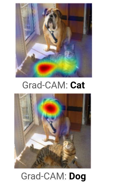
We might expect the CNN to rely on different morphological features for recognizing different classes. If these essential features are altered, then the classification might change dramatically. Therefore, we need to look at features for which the gradient (corresponding to a given feature) is large, and this can be accomplished by visualizing the gradient-weighted class activation map (Grad-CAM). This work is detailed in "Grad-CAM: Visual Explanations from Deep Networks via Gradient-based Localization," by Selvaraju et al. (2016).

Pytorch automatically computes gradients during the backwards pass for each (trainable) layer. However, it doesn't store them, so we need to make use of the hook functionality in order to save them on the forward pass (activations) and backward pass (gradients). The essential Pytorch code is shown below (adapted from the Fastai book).
class HookActivation():
    def __init__(self, target_layer):
        """Initialize a Pytorch hook using `hook_activation` function."""

        self.hook = target_layer.register_forward_hook(self.hook_activation)

    def hook_activation(self, target_layer, activ_in, activ_out):
        """Create a copy of the layer output activations and save
        in `self.stored`.
        """
        self.stored = activ_out.detach().clone()

    def __enter__(self, *args):
        return self

    def __exit__(self, *args):
        self.hook.remove()


class HookGradient():
    def __init__(self, target_layer):
        """Initialize a Pytorch hook using `hook_gradient` function."""

        self.hook = target_layer.register_backward_hook(self.hook_gradient)

    def hook_gradient(self, target_layer, gradient_in, gradient_out):
        """Create a copy of the layer output gradients and save
        in `self.stored`.
        """
        self.stored = gradient_out[0].detach().clone()

    def __enter__(self, *args):
        return self

    def __exit__(self, *args):
        self.hook.remove()
Note that the two classes are almost the same, and that all of the business logic can be boiled down to:
- define a hook function (e.g.,
hook_gradient) that captures the relevant output from a model layer - register a forward or backward hook using this function
- define a Python context using
__enter__and__exit__so that we don't waste memory and can easily call the hooks likewith(HookGradient) as hookg: [...]
We're interested in the final convolutional layer, as the early layers may have extremely vague features that that may not correspond specifically to any one class.
target_layer = learn.model[-4]

learn.model
We also need to operate on a single image at a time. (I think we can technically use a mini-batch of images, but then we'll end up with a huge tensor of gradients!) Let's target this nice-looking galaxy.
img = PILImage.create(f'{ROOT}/images/1237665024900858129.jpg')
img.show()
We can see that the model is incredibly confident that this image is of a high-metallicity galaxy.
learn.predict(img)
However, learn.predict() is doing a lot of stuff under the hood, and we want to attach hooks to the model while it's doing all that. So we'll walk through this example step-by-step.
First, we need to apply all of the item_tfms and batch_tfms (like cropping the image, normalizing its values, etc) to this test image. We can put this image into a batch and then retrieve it (along with non-existent labels) using first(dls.test_dls([img])).
We use dls.train.decode() to process these transforms, and pass it (the first element, and first batch) into a TensorImage which can be shown the same was as a PILImage.
x, = first(dls.test_dl([img]))

x_img = TensorImage(dls.train.decode((x,))[0][0])
x_img.show()
Next, we want to generate the Grad-CAM maps. We can produce one for each class, so let's double-check dls.vocab to make sure we know the mapping between integers and high or low metallicity classes. It turns out that 0 corresponds to high, 1 corresponds to low. (We also could have figured it out from the output of learn.predict() above.)
dls.vocab
At this point, we can simply apply the hooks and save the stored values into other variables.
- During the forward pass, we want to put the model into eval mode and stick the image onto the GPU:
learn.model.eval()(x.cuda()). We can then save the activation inact. - We then need to do a backwards pass to compute gradients with respect to one of the class labels. If we want gradients with respect to the low-metallicity class, then we would call
output[0, 1].backward()(note that this 0 references the lone example in the mini-batch). We can store the gradient ingrad. - We might also find it helpful to get the class probabilities, which we temporarily saved in
output. We can get rid of their gradients and store the two values inp0andp1, the low-z and high-z probabilities (which sum up to one).
# low-metallicity
class_Z = 1

with HookGradient(target_layer) as hookg:
    with HookActivation(target_layer) as hook:
        output = learn.model.eval()(x.cuda())
        act = hook.stored
    output[0, class_Z].backward()
    grad = hookg.stored
    p0, p1 = output.cpu().detach()[0]
Finally, computing the Grad-CAM map is super easy! We average the gradients across the spatial axes (leaving only the "feature" axis) and then take the inner product with the activation maps. In the language of mathematics, we are computing
$$ \sum_{k} \frac{\partial y}{\partial \mathbf{A}^{(k)}_{ij}} \left [ \frac{1}{N_i N_j}\sum_{i,j} \mathbf{A}^{(k)}_{ij} \right ],$$
for the $k$ feature maps, $\mathbf{A}^{(k)}_{i,j}$, and the target class $y$. Note that the feature maps have shape $N_i \times N_j$, which ends up in the denominator as a constant, but this just gives us an arbitrary scaling factor. Finally, we stop Pytorch from computing any more gradients and pop it off the GPU with .detach() and .cpu(). We can then plot the map below.
w = grad[0].mean(dim=(1,2), keepdim=True)
gradcam_map = (w * act[0]).sum(0).detach().cpu()
Interesting! Looks like it has highlighted the outer regions of the galaxy. Let's also visualize the high-metallicity parts of the image using the same exact code (except, of course, switching class_Z = 0 to class_Z = 1):
Putting it together
Cool, so now we know how this all works! However, we should actually take only the positive contributions of the Grad-CAM map, because activations are passed through a ReLU layer in the CNN. We can do this by calling torch.clamp(). Since matplotlib imshow() rescales the colormap anyway, the result is that we'll see less of the lower-valued (darker) portions of the Grad-CAM map, but the higheest-valued (brighter) parts will not change.
We will shove all this into a function, plot_gradcam, which computes the Grad-CAM maps for low and high metallicity labels, organizes the matplotlib plotting, and returns the figure, axes, and CNN probabilities.
def plot_gradcam(x, learn, hooked_layer, size=96):

    fig, axes = plt.subplots(1, 3, sharey=True, figsize=(8.5, 3), dpi=150)

    x_img = TensorImage(dls.train.decode((x,))[0][0])


    for i, ax in zip([0, 2, 1], axes):

        if i == 0:
            x_img.show(ax=ax)
            ax.set_axis_off()
            continue

        with HookGradient(hooked_layer) as hookg:
            with HookActivation(hooked_layer) as hook:
                output = learn.model.eval()(x.cuda())
                act = hook.stored
            output[0, i-1].backward()
            grad = hookg.stored
            p_high, p_low = output.cpu().detach()[0]

        w = grad[0].mean(dim=(1,2), keepdim=True)
        gradcam_map = (w * act[0]).sum(0).detach().cpu()

        # thresholding to account for ReLU
        gradcam_map = torch.clamp(gradcam_map, min=0)

        x_img.show(ax=ax)
        ax.imshow(
            gradcam_map, alpha=0.6, extent=(0, size, size,0),
            interpolation='bicubic', cmap='inferno'
        )
        ax.set_axis_off()

    fig.tight_layout()
    fig.subplots_adjust(wspace=0.02)

    return (fig, axes, *(np.exp([p_low, p_high]) / np.exp([p_low, p_high]).sum()))
And now we can plot it! It looks much better now that we've applied the ReLU. I have also added a few extra captions so that we can see the object ID and CNN prediction probabilities.
We can see not only why the CNN (confidently) classified this galaxy as a high-metallicity system, i.e. its bright central region, but also which parts of the image were most compelling for it to be classified as a low-metallicity galaxy, even though it didn't make this prediction! Here, we see that it has highlighted the far-outer blue spiral arms of this galaxy.
A few more examples
Since we've invested this effort into making the plot_gradcam() function, let's generate some more pretty pictures. We can grab some random galaxies from the validation set between the redshifts 0.05 < z < 0.08 (i.e., typical galaxy redshifts), and process them using the trained CNN and Grad-CAM.
val_df = dls.valid.items

objids = val_df[(0.05 < val_df.z) & (val_df.z < 0.08)].sample(5, random_state=seed).objID
Conclusions
I hope that you've enjoyed this journey through data visualization techniques using fast.ai! One of the goals was to convince you that convolutional neural networks can be interpretable, and that methods like Grad-CAM are crucial for understanding what a CNN has learned. Since the neural network makes more accurate predictions than any human, we can gain invaluable knowledge by observing what the model focuses on, potentially leading to new insights in astronomy!
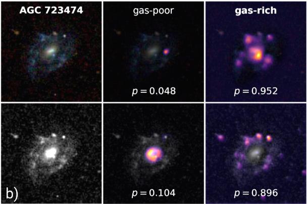
If you're interested in some academic discussion of this sort of topic, then I encourage you to check out my most recent paper, "Connecting optical morphology, environment, and HI mass fraction for low-redshift galaxies using deep learning", which delves into a closely related topic. In this work, I use pattern recognition classifier combined with a highly optimized CNN regression model to estimate the gas content of galaxies with state-of-the-art results! Grad-CAM makes an appearance in Figure 11, and is even used for visual attribution in monochromatic images (see below). The paper has just been accepted to the Astrophysical Journal (ApJ), and is currently in press, but you can view the semi-final version on arXiv now!
