Training a deep CNN to learn about galaxies in 15 minutes
Let's train a deep neural network from scratch! In this post, I provide a demonstration of how to optimize a model in order to predict galaxy metallicities using images, and I discuss some tricks for speeding up training and obtaining better results.
- Predicting metallicities from pictures: obtaining the data
- Organizing the data using the fastai DataBlock API
- Neural network architecture and optimization
- Evaluating our results
- Summary
Predicting metallicities from pictures: obtaining the data
In my previous post, I described the problem that we now want to solve. To summarize, we want to train a convolutional neural network (CNN) to perform regression. The inputs are images of individual galaxies (although sometimes we're photobombed by other galaxies). The outputs are metallicities, $Z$, which usually take on a value between 7.8 and 9.4.
The first step, of course, is to actually get the data. Galaxy images can be fetched using calls to the Sloan Digital Sky Survey (SDSS) SkyServer getJpeg cutout service via their RESTful API. For instance, this URL grabs a three-channel, $224 \times 224$-pixel JPG image:
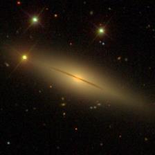
Galaxy metallicities can be obtained from the SDSS SkyServer using a SQL query and a bit of JOIN magic. All in all, we use 130,000 galaxies with metallicity measurements as our training + validation data set.
The code for the original published work (Wu & Boada 2019) can be found in my Github repo. However, this code (from 2018) used fastai version 0.7, and I want to show an updated version using the new and improved fastai version 2 codebase. Also, some of the "best practices" for deep learning and computer vision have evolved since then, so I'd like to highlight those updates as well!
Suppose that we now have a directory full of galaxy images, and a csv file with the object identifier, coordinates, and metallcity for each galaxy. The csv table can be read using Pandas, so let's store that in a DataFrame df. We can take a look at five random rows of the table by calling df.sample(5):
This means that a galaxy with objID 1237654601557999788 is located at RA = 137.603036 deg, Dec = 3.508882 deg, and has a metallicity of $Z$ = 8.819281. Our directory structure is such that the corresponding image is stored in {ROOT}/images/1237660634922090677.jpg, where ROOT is the path to project repository.
A tree-view from our {ROOT} directory might look like this:
.
├── data
│   └── master.csv
├── images
│   ├── 1237654601557999788.jpg
│   ├── 1237651067353956485.jpg
│   └── [...]
└── notebooks
    └── training-a-cnn.ipynb
We are ready to set up our DataBlock, which is a core fastai construct for handling data. The process is both straightforward and extremely powerful, and comprises a few steps:
- Define the inputs and outputs in the
blocksargument - Specify how to get your inputs (
get_x) and outputs (get_y) - Decide how to split the data into training and validation sets (
splitter) - Define any CPU-level transformations (
item_tfms) and GPU-level transformations (batch_tfms) used for preprocessing or augmenting your data.
Before going into the details for each component, here is the code in action:
dblock = DataBlock(
    blocks=(ImageBlock, RegressionBlock),
    get_x=ColReader(['objID'], pref=f'{ROOT}/images/', suff='.jpg'),
    get_y=ColReader(['metallicity']),
    splitter=RandomSplitter(0.2),
    item_tfms=[CropPad(144), RandomCrop(112)],
    batch_tfms=aug_transforms(max_zoom=1., flip_vert=True, max_lighting=0., max_warp=0.) + [Normalize],
)
Okay, now let's take a look at each part.
First, we want to make use of the handy ImageBlock class for handling our input images. Since we're using galaxy images in the JPG format, we can rely on the PIL backend of ImageBlock to open the images efficiently. If, for example, we instead wanted to use images in the astronomical FITS format, we could extend the TensorImage class and define the following bit of code:
#collapse-hide
class FITSImage(TensorImage):
    @classmethod
    def create(cls, filename, chans=None, **kwargs) -> None:
        """Create FITS format image by using Astropy to open the file, and then
        applying appropriate byte swaps and flips to get a Pytorch Tensor.
        """
        return cls(
            torch.from_numpy(
                astropy.io.fits.getdata(fn).byteswap().newbyteorder()
            )
            .flip(0)
            .float()
        )

    def show(self, ctx=None, ax=None, vmin=None, vmax=None, scale=True, title=None):
        """Plot using matplotlib or your favorite program here!"""
        pass

FITSImage.create = Transform(FITSImage.create)

def FITSImageBlock():
    """A FITSImageBlock that can be used in the fastai DataBlock API.
    """
    return TransformBlock(partial(FITSImage.create))
For our task, the vanilla ImageBlock will suffice.
We also want to define an output block, which will be a RegressionBlock for our task (note that it handles both single- and multi-variable regression). If, for another problem, we wanted to do a categorization problem, then we'd intuitively use the CategoryBlock. Some other examples of the DataBlock API can be found in the documentation.
We can pass in these arguments in the form of a tuple: blocks=(ImageBlock, RegressionBlock).
Next, we want to be able to access the table, df, which contain the columns objID and metallicity. As we've discussed above, each galaxy's objID can be used to access the JPG image on disk, which is stored at {ROOT}/images/{objID}.jpg. Fortunately, this is easy to do with the fastai ColumnReader method! We just have to supply it with the column name (objID), a prefix ({ROOT}/images/), and a suffix (.jpg); since the prefix/suffix is only used for file paths, the function knows that the file needs to be opened (rather than interpreting it as a string). So far we have:
get_x=ColReader(['objID'], pref=f'{ROOT}/images/', suff='.jpg')
The targets are stored in metallicity, so we can simply fill in the get_y argument:
get_y=ColReader(['metallicity'])
(At this point, we haven't yet specified that df is the DataFrame we're working with. The DataBlock object knows how to handle the input/output information, but isn't able to load it until we provide it with df -- that will come later!)
For the sake of simplicity, we'll just randomly split our data set using the aptly named RandomSplitter function. We can provide it with a number between 0 and 1 (corresponding to the fraction of data that will become the validation set), and also a random seed if we wish. If we want to set aside 20% of the data for validation, we can use this:
splitter=RandomSplitter(0.2, seed=56)
Next, I'll want to determine some data augmentation transformations. These are handy for varying our image data: crops, flips, and rotations can be applied at random using fastai's aug_transforms() in order to dramatically expand our data set. Even though we have >100,000 unique galaxy images, our CNN model will contain millions of trainable parameters. Augmenting the data set will be especially valuable for mitigating overfitting.
Translations, rotations, and reflections to our images should not change the properties of our galaxies. However, we won't want to zoom in and out of the images, since that might impact CNN's ability to infer unknown (but possibly important) quantities such as the galaxies' intrinsic sizes. Similarly, color shifts or image warps may alter the star formation properties or stellar structures of the galaxies, so we don't want to mess with that.
We will center crop the image to $144 \times 144$ pixels using CropPad(), which reduces some of the surrounding black space (and other galaxies) near the edges of the images. We will then apply a $112 \times 112$-pixel RandomCrop() for some more translational freedom. This first set of image crop transformations, item_tfms, will be performed on images one by one using a CPU. Afterwards, the cropped images (which should all be the same size) will be loaded onto the GPU. At this stage, data augmentation transforms will be performed along with image normalization, which rescales the intensities in each channel so that they have zero mean and unit variance. The second set of transformations, batch_tfms, will be applied one batch at a time on the GPU.
item_tfms=[CropPad(144), RandomCrop(112)]
batch_tfms=aug_transforms(max_zoom=1., flip_vert=True, max_lighting=0., max_warp=0.) + [Normalize]
Normalize will pull the batch statistics from your images, and apply it any time you load in new data (see below). Sometimes this can lead to unintended consequences, for example, if you’re loading in a test data set which is characterized by different image statistics. In that case, I recommend saving your batch statistics and then using them later, e.g., Normalize.from_stats(*image_statistics).
We've now gone through each of the steps, but we haven't yet loaded the data! ImageDataLoaders has a class method called from_dblock() that loads everything in quite nicely if we give it a data source. We can pass along the DataBlock object that we've constructed, the DataFrame df, the file path ROOT, and a batch size. We've set the batch size bs=128 because that fits on the GPU, and it ensures speedy training, but I've found that values between 32 and 128 often work well.
dls = ImageDataLoaders.from_dblock(dblock, df, path=ROOT, bs=128)
Once this is functional, we can view our data set! As we can see, the images have been randomly cropped such that the galaxies are not always in the center of the image. Also, much of the surrounding space has been cropped out.
dls.show_batch(nrows=2, ncols=4)
Pardon the excessive number of significant figures. We can fix this up by creating custom classes extending Transform and ShowTitle, but this is beyond the scope of the current project. Maybe I'll come back to this in a future post!
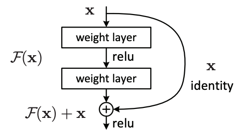
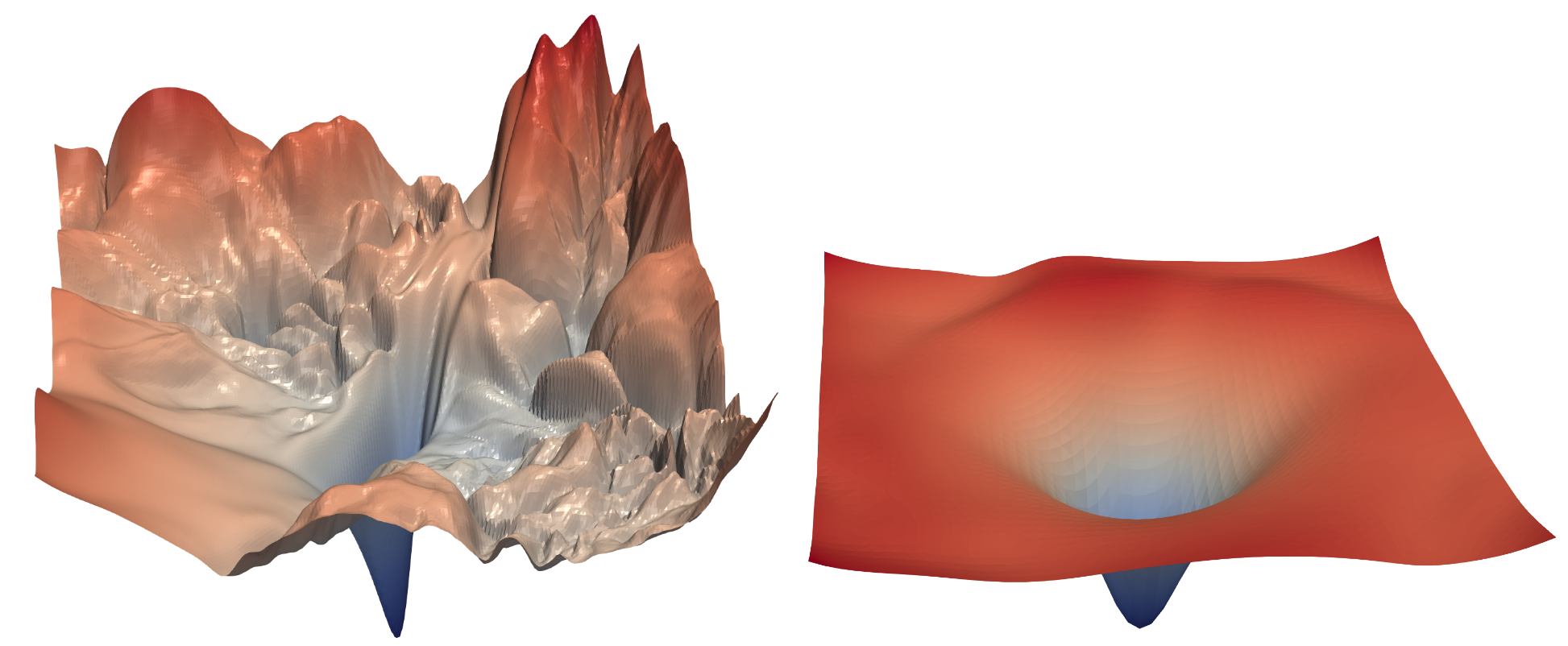
There's no way that I can describe all of the tweaks and improvements that machine learning researchers have made in the past couple of years, but I'd like to highlight a few that really help out our cause. We need to use some kind of residual CNNs (or resnets), introduced by Kaiming He et al. (2015). Resnets outperform previous CNNs such as the AlexNet or VGG architectures because they can leverage gains from "going deeper" (i.e., by extending the resnets with additional layers). The paper is quite readable and interesting, and there are plenty of other works explaining why resnets are so successful (e.g., a blog post by Anand Saha and a deep dive into residual blocks by He et al.).
In fastai, we can instantiate a 34-layer enhanced resnet model by using model = xresnet34(). We could have created a 18-layer model with model = xresnet18(), or even defined our own custom 9-layer resnet using
xresnet9 = XResNet(ResBlock, expansion=1, layers=[1, 1, 1, 1])
model = xresnet9()
But first, we need to set the number of outputs. By default, these CNNs are suited for the ImageNet classification challenge, and so there are 1000 outputs. Since we're performing single-variable regression, the number of outputs (n_out) should be 1. Our DataLoaders class, dls, already knows this and has stored the value 1 in dls.c.
Okay, let's make our model for real:
model = xresnet34(n_out=dls.c, sa=True, act_cls=MishCuda)
So why did I say that we're using an "enhanced" resnet -- an "xresnet"? And what does sa=True and act_cls=MishCuda mean? I'll describe these tweaks below.
The "bag of tricks" paper by Tong He et al. (2018) summarizes many small tweaks that can be combined to dramatically improve the performance of a CNN. They describe several updates to the resnet model architecture in Section 4 of their paper. The fastai library takes these into account, and also implements a few other tweaks, in order to increase performance and speed. I've listed some of them below:
- The CNN stem (first few layers) is updated using efficient $3 \times 3$ convolutions rather than a single expensive layer of $7\times 7$ convolutions.
- Residual blocks are changed so that $1 \times 1$ convolutions don't skip over useful information. This is done by altering the order of convolution strides in one path of the downsampling block, and adding a pooling layer in the other path (see Figure 2 of He et al. 2018).
- The model concatenates the outputs of both AveragePool and MaxPool layers (using
AdaptiveConcatPool2d) rather than using just one.
Some of these tweaks are described in greater detail in Chapter 14 of the fastai book, "Deep Learning for Coders with fastai and Pytorch" (which can be also be purchased on Amazon).
The concept of attention has gotten a lot of, well, attention in deep learning, particularly in natural language processing (NLP). This is because the attention mechanism is a core part of the Transformer architecture, which has revolutionized our ability to learn from text data. I won't cover the Transformer architecture or NLP in this post, since it's way out of scope, but suffice it to say that lots of deep learning folks are interested in this idea.
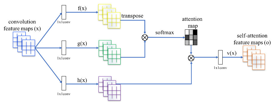
The attention mechanism allows a neural network layer to encode interactions from inputs on scales larger than the size of a typical convolutional filter. Self-attention is simply when these relationships, encoded via a query/key/value system, are applied using the same input. As a concrete example, self-attention added to CNNs in our scenario -- estimating metallicity from galaxy images -- may allow the network to learn morphological features that often require long-range dependencies, such as the orientation and position angle of a galaxy.
In fastai, we can set sa=True when initializing a CNN in order to get the self-attention layers!
Another way to let a CNN process global information is to use Squeeze-and-Excitation Networks, which are also included in fastai. Or, one could even entirely replace convolutions with self-attention. But we're starting to get off-topic...
Typically, the Rectified Linear Unit (ReLU) is the non-linear activation function of choice for nearly all deep learning tasks. It is both cheap to compute and simple to understand: ReLU(x) = max(0, x).
That was all before Diganta Misra introduced us to the Mish activation function -- as an undergraduate researcher! He also wrote a paper and summarizes some of the reasoning behind it in a forum post. Less Wright, from the fastai community, shows that it performs extremely well in several image classification challenges. I've also found that Mish is perfect as a drop-in replacement for ReLU in regression tasks.
The intuition behind the Mish activation function's success is similar to the reason why resnets perform so well: the loss landscape becomes smoother and thereby easier to explore. ReLU is non-differentiable at the origin, causing steep spikes in the loss. Mish resembles another activation function, GELU (or SiLU), in that neither it nor its derivative is monotonic; this seems to lead to more complex and nuanced behavior during training. However, it's not clear (from a theoretical perspective) why such activation functions empirically perform so well.
Although Mish is a little bit slower than ReLU, a CUDA implementation helps speed things up a bit. We need to pip install it and then import it with from mish_cuda import MishCuda. Then, we can substitute it into the model when initializing our CNN using act_cls=MishCuda.
Next we want to select a loss function. The mean squared error (MSE) is suitable for training the network, but we can more easily interpret the root mean squared error (RMSE). We need to create a function to compute the RMSE loss between predictions p and true metalllicity values y.
(Note that we use .view(-1) to flatten our Pytorch Tensor objects since we're only predicting a single variable.)
def root_mean_squared_error(p, y):
    return torch.sqrt(F.mse_loss(p.view(-1), y.view(-1)))
Around mid-2019, we saw two new papers regarding the stability of training neural networks: LookAhead and Rectified Adam (RAdam). Both papers feature novel optimizers that address the problem of excess variance during training. LookAhead mitigates the variance problem by scouting a few steps ahead, and then choosing how to optimally update the model's parameters. RAdam adds a term while computing the adaptive learning rate in order to address training instabilities (see, e.g., the original Adam optimizer).
Less Wright quickly realized that these two optimizers could be combined. His ranger optimizer is the product of these two papers (and now also includes a new tweak, gradient centralization, by default). I have found ranger to give excellent results using empirical tests.
So, now we'll put everything together in a fastai Learner object:
learn = Learner(
    dls,
    model,
    opt_func=ranger,
    loss_func=root_mean_squared_error
)
Fastai offers a nice feature for determining an optimal learning rate, taken from Leslie Smith (2015). All we have to do is call learn.lr_find().
The idea is to begin feeding your CNN batches of data, while exponentially increasing learning rates (i.e., step sizes) and monitoring the loss. At some point the loss will bottom out, and then begin to increase and diverge wildly, which is a sign that the learn rate is now too high.
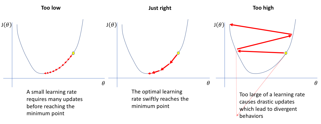
Generally, before the loss starts to diverge, the learning rate will be suitable for the loss to steadily decrease. We can generally read an optimal learning rate off the plot -- the suggested learning rate is around $0.03$ (since that is about an order of magnitude below the learning rate at which the loss "bottoms out" and is also where the loss is decreasing most quickly). I tend to choose a slightly lower learning rate (here I'll select $0.01$), since that seems to work better for my regression problems.
learn.lr_find()
Finally, now that we've selected a learning rate ($0.01$), we can train for a few epochs. Remember that an epoch is just a run-through using all of our training data (and we send in one batch of 64 images at a time). Sometimes, researchers simply train at a particular learning rate and wait until the results converge, and then lower the learning rate in order for the model to continue learning. This is because the model needs some serious updates toward the beginning of training (given that it has been initialized with random weights), and then needs to start taking smaller steps once its weights are in the right ballpark. However, the learning rate can't be too high in th beginning, or the loss will diverge! Traditionally, researchers will select a safe (i.e., low) learning rate in the beginning, which can take a long time to converge.
Fastai offers a few optimization schedules, which involve altering the learning rate over the course of training. The two most promising are called fit_flat_cos and fit_one_cycle (see more here). I've found that fit_flat_cos tends to work better for classification tasks, while fit_one_cycle tends to work better for regression problems. Either way, the empirical results are fantastic -- especially coupled with the Ranger optimizer and all of the other tweaks we've discussed.
learn.fit_one_cycle(7, 1e-2)
Here we train for only seven epochs, which took under 14 minutes of training on a single NVIDIA P100 GPU, and achieve a validation loss of 0.086 dex. In our published paper, we were able to reach a RMSE of 0.085 dex in under 30 minutes of training, but that wasn't from a randomly initialized CNN -- we were using transfer learning then! Here we can accomplish similar results, without pre-training, in only half the time.
We can visualize the training and validation losses. The x-axis shows the number of training iterations (i.e., batches), and the y-axis shows the RMSE loss.
learn.recorder.plot_loss()
plt.ylim(0, 0.4);
Finally, we'll perform another round of data augmentation on the validation set in order to see if the results improve. This can be done using learn.tta(), where TTA stands for test-time augmentation.
preds, trues = learn.tta()
Note that we'll want to flatten these Tensor objects and convert them to numpy arrays, e.g., preds = np.array(preds.view(-1)). At this point, we can plot our results. Everything looks good!
It appears that we didn't get a lower RMSE using TTA, but that's okay. TTA is usually worth a shot after you've finished training, since evaluating the neural network is relatively quick.
In summary, we were able to train a deep convolutional neural network to predict galaxy metallicity from three-color images in under 15 minutes. Our data set contained over 100,000 galaxies, so this was no easy feat! Data augmentation, neural network architecture design, and clever optimization tricks were essential for improving performance. With these tools in hand, we can quickly adapt our methodology to tackle many other kinds of problems!
fastai version 2 is a powerful high-level library that extends Pytorch and is easy to use/customize. As of November 2020, the documentation is still a bit lacking, but hopefully will continue to mature. One big takeaway is that fastai, which is all about democratizing AI, makes deep learning more accessible than ever before.
Acknowledgments: I want to thank fastai core development team, Jeremy Howard and Sylvain Gugger, as well as other contributors and invaluable members of the community, including Less Wright, Diganta Misra, and Zachary Mueller. I also want to acknowledge Google for their support via GCP credits for academic research. Finally, I want to give a shout out to Steven Boada, my original collaborator and co-author on our paper.
Last updated: November 16, 2020