Re-envisioning Euclid Galaxy Morphology

With the Euclid and Roman Space Telescope missions ready to image billions of galaxies, we’ll need data-driven methods to find new, rare phenomena that exist outside human-defined taxonomies! Sparse Autoencoders (SAEs) can be that discovery engine, surfacing interpretable features in modern galaxy surveys. This blog post highlights some preliminary results from our tiny NeurIPS ML4PS workshop paper, jointly led by Mike Walmsley and me. Read the paper here.

Galaxy Morphologies in Euclid

Euclid¹ is now delivering crisp, space-based imaging for millions of galaxies. Among the many scientific results presented in their Q1 (“Quick Data Release 1”) is a citizen science analysis of galaxy morphologies presented by Mike Walmsley et al. This paper presents not only GalaxyZoo (GZ) volunteer classifications according to a decision tree — i.e., Is this galaxy featured? Does it have spiral arms? How many? — but also a foundation model (Zoobot) fine-tuned for predicting these decision classes on the Euclid galaxy dataset. You can check out the Zoobot v2.0 blog post and download it via Github.

But Zoobot follows a supervised approach: we’ve delineated the taxonomy into which galaxies must fit. By definition, this CNN learns representations that enable it to accurately describe galaxy according to the GZ categories. Can we get a neural network model to represent galaxies outside of this taxonomy?

Yes! Our first result from this paper is to present a Masked Autoencoder (MAE) that learns galaxy imaging via self-supervised representations. Our MAE chops up images into 8×8 patches, and consists of a custom vision transformer (ViT) encoder with ~30M parameters, and a three-layer decoder. To get a sense of how it works, I highly recommend you checking out the interactive demo built by Mike: https://huggingface.co/spaces/mwalmsley/euclid_masked_autoencoder

Even when you remove 90% of the pixels of a Euclid image, the MAE can learn to reconstruct the rest of the image extraordinarily well. Honestly, it does far better than any human can. And not only does it work for galaxy images, but the MAE also learns to reconstruct bright stars and other objects in the Euclid RR2 dataset.

Principal Components of Galaxy Image Embeddings

Okay, so we have trained models, which means that we can encode Euclid images into Zoobot (supervised; d=640) and/or MAE (self-supervised; d=384) embeddings. How do we interpret these learned embedding vectors?

A good starting point is to use PCA (principal components analysis); the top PCs should summarize most of the variation in each dataset. It’s worth emphasizing that the supervised (Zoobot) and self-supervised (MAE) models are trained on different datasets: the Zoobot dataset comprises ~380k well-resolved galaxy images from Euclid, whereas the MAE dataset comprises >3M Euclid images of galaxies, stars, artifacts, etc. Thus, it is not possible to make an apples-to-apples comparison between these two datasets or their embeddings.

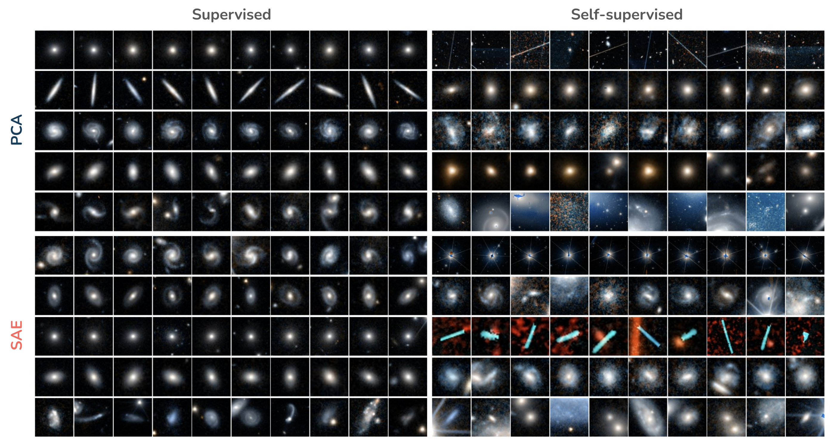
The figure above, copied from Figure 2 in the paper, displays top image examples for the first five PCs for Zoobot (left) and MAE (right) model embeddings. Some interesting notes:

• For the supervised Zoobot embeddings, our first few PCs are well-aligned with the first few nodes of the GZ decision tree.
  • For example, the first PC mirrors the first GZ question of whether the galaxy is smooth or featured with Spearman r≈0.85.
  • The next questions align with whether a featured galaxy has a disk that is seen edge-on, or has spiral arms, or has a prominent bulge, etc.
  • Note that PCs can have both positive and negative coefficient, so the first PC with a very positive coefficient would characterize a very smooth (e.g. spheroidal) galaxy, while a very negative coefficient would characterize a stronlgy featured (e.g. spiral arms) galaxy!
• For the self-supervised MAE embeddings, the representations are totally different than before.
  • In several of the top PCs, we find cosmic ray hits or other imaging artifacts.
  • We think these dominate much of the MAE latent space because it’s fundamentally challenging to reconstruct images with imaging artifacts!
  • Galaxies also appear in here, although individual PCs do not align nearly as strongly to the GZ categories.

PCA is nice because it rank-orders features by how much they explain the variance in the embedding vectors. But what if the features you want require non-linear combinations of embeddings? Or what if your original embeddings are noisy, so each PC depends on all inputs — this might result in uninterpretable features.

Sparse Autoencoders for Interpretability and Discovery

For this reason, we chose to use a sparse coding method, Matryoshka Sparse Autoencoders (SAEs), to discover features! They’re extremely simple: embeddings get fed into a single layer decoder (with ReLU activation), wherein only a few neurons are allowed to be active.² From these sparse activations, a single-layer decoder (i.e. a projection matrix) learns to reconstruct the original embeddings. Because the latent activations are sparse, the SAE must use only a few neurons to reconstruct each given input (i.e., the original images), which results in more interpretable features. Possibly even monosemantic features — that is, instead of a many-to-many mapping between neuron activations and semantic concepts, we can use SAEs to recover a one-to-one mapping between activations and concepts.

Or so the story goes. Famously, Anthropic found a Golden Gate Bridge feature in Claude that activates on both text and images! But… while SAEs are sure to learn sparse, non-linear combinations in an overcomplete space, we don’t actually have mathematical guarantees that SAEs will find monosemantic or disentangled features. What does monosemanticity even really mean? Should galaxies with Sersic indices of 2.1 activate a different feature than galaxies with Sersic indices of 2.2? Indeed, there is significant evidence that SAEs do not fare as well as linear probes for already known features, leading some research teams to focus on other topics in mechanistic interpretability.

Anyway, let’s just see what happens. Take a look at the figure above again, and now focus on the bottom panels. These now show the first five SAE features, ranked in order of how frequently they are activated. For the supervised example (on the lower left), we can see reasonably coherent/interpretable features: two-armed spirals, ringed galaxies, spheroidal galaxies, elliptical galaxies, and objects with tidal features, clumps, or companions. (This last one is the least monosemantic, but it’s intriguing because each of those features can be indicative of galaxy–galaxy interactions or mergers!) For the self-supervised MAE (on the lower right), we also see some consistency in SAE-extracted features. Huh!

We then quantify how well the PCA and SAE features align with GZ features, using the Spearman rank correlation coefficient I discussed earlier. Again, we shouldn’t compare between the supervised and self-supervised models, but we can now compare PCA and SAE features! And we find a clear winner: SAE features are typically more aligned with the GZ taxonomy!

Qualitatively, we also find that the SAE can surface interesting features. This is most evident in the features extracted from Zoobot embeddings, where we know the supervised training objective. For example, we find examples of ring galaxies or dust lanes in edge-on disk galaxies — visually clear signatures of coherent features that aren’t in the training objective. The MAE model is probably full of interesting SAE-extracted features, too, but some of them are definitely challenging to interpret.

Anyway, there’s much more to say, but at this point the blog post might be comparable in length to our workshop paper! Just go read the paper, or try it out using our code — I’d love to hear what you think!