Galaxy environments and graph neural networks

This post discusses how graph neural networks (GNNs) can model the galaxy–halo connection within its large-scale surroundings. Dark matter structures, which seem to account for most of the mass in the Universe, can be represented as nodes in a cosmic graph. But dark matter—which solely interacts via gravitation—is also much easier to simulate than the messy baryons, whose magnetohydrodynamics are computationally expensive. By exploiting the representational power of GNNs, can we predict galaxies’ baryonic properties purely using simple dark matter-only simulations? Yes we can!

Note: this post is a continuation of a previous introduction to GNNs in astrophysics. Special thanks to Christian Kragh Jespersen,¹ who opened my eyes to the incredible power of GNNs for astrophysics! He also has several papers showing that graphs provide strong representations for galaxy merger trees (see here and follow-up here).

The galaxy–halo connection

In the ΛCDM cosmology, galaxies live in dark matter subhalos² (see, e.g., the review by Wechsler & Tinker). While dark matter dominates the mass content of the Universe, we can only directly observe the luminous signatures from galaxies that reside within. Our goal is to determine whether galaxy properties, such as its total stellar mass, can be predicted purely from dark matter simulations.

To solve this problem 20 years ago, a technique called “subhalo abundance matching” was proposed. The goal is to connect simulated dark matter subhalos to galaxy populations based on the latter’s stellar masses (or luminosities). By rank-ordering the subhalo masses and assigning them to rank-ordered galaxy stellar masses, abundance matching imposes a monotonic relationship between the two populations.

This simple technique is capable of connecting galaxies to their host halos. However, it also assumes that galaxy evolution is not dictated by anything but the dark matter halo properties. Therefore, abundance matching fails to account for each galaxy’s large-scale environment!

To the cosmic web and beyond

We’ve known for a long time that galaxy properties depend on their surroundings (see, e.g., Dressler’s famous 1980 paper). The exact nature of how this plays out is uncertain; does galaxy environment induce different mass accretion or merger rate? Do overdense environments superheat or exhaust cool gas needed to fuel star formation? Or do large-scale tidal torques alter galaxy properties over cosmic timescales? We don’t really know the answer!³ But empirically, we do know that the galaxy–halo connection also varies with environment.

Overdensity

Some attempts have been made to account for galaxy environment. For example, “overdensity” is a common parameterization of the mass density on large scales (see, e.g., Blanton et al. 2006). Whereas a typical galaxy’s gravitational influence extends to a few hundred kpc, the overdensity can quantify the average density out to many Mpc. However, by taking a simple average over all mass in this spherical volume, the overdensity parameter is not sensitive to local variations in mass.

DisPerSE

Another popular technique called DisPerSE aims to measure topological structures in the cosmic web, e.g., voids, filaments, sheets, and clusters. DisPerSE is short for Discrete Persistent Structure Extractor, and the general intuition for how it works is by: (1) computing a density field from the simulation particles, (2) identifying critical points of the field like minima, saddle points, and maxima, (3) tracing out the “skeleton” between critical points, and (4) filtering features by their topological persistence, ensuring only robust, noise-resistant structures are kept. We can thus describe galaxy environment by using the distances to these DisPerSE features.

Cosmic GNNs

Christian and I recognized that the entire simulated volume of galaxies could be represented a single cosmic graph, and subsequently modeled via GNNs! You can see a visualization of this below (Figure 1 of Wu & Jespersen 2023).

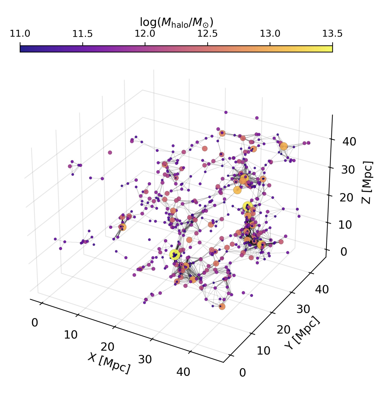
We used matched runs of the Illustris TNG 300 dark matter only (DMO) + hydrodynamic simulations, i.e., the DMO simulation can only form dark matter (sub)halos, whereas the hydrodynamic run begins with the same initial conditions and forms similar (sub)halos as its DMO counterpart, but also includes messy baryonic physics. This means that we can map hydrodynamic galaxy predictions using a cosmic graph constructed from DMO simulations!

We treat each subhalo as a node in this cosmic graph, and specify two DMO node features: the total subhalo mass (M_subhalo) and the maximum circular velocity (V_max).

To determine the graph connectivity, we imposed a constant linking length. Pairs of galaxies “know” about each other if they have smaller separations than the linking length, so we connect those pairs of nodes with graph edges. We also compute six edge features using the nodes’ 3D positions and 3D velocities; these edge features record the geometry of the system in a E(3) group-invariant way.

As for the GNN model architecture, we use a graph network analogous to those described by Battaglia et al. 2018 that we had seen successfully applied in cosmology. If you really want to see the code, take a look here.

So… how do overdensity, DisPerSE, and GNNs compare?

To cut to the chase: GNNs dominate the competition when it comes to predicting galaxy stellar masses from DMO simulations.

The figure below shows how different environmental indicators, quantified over various distance scales, affect the prediction error on M_star. Lower error is better, and you can clearly see how GNNs (purple) surpass all other methods once they’re given information on > 1 Mpc length scales. (Figure adapted from Wu, Jespersen, & Wechsler 2024.)

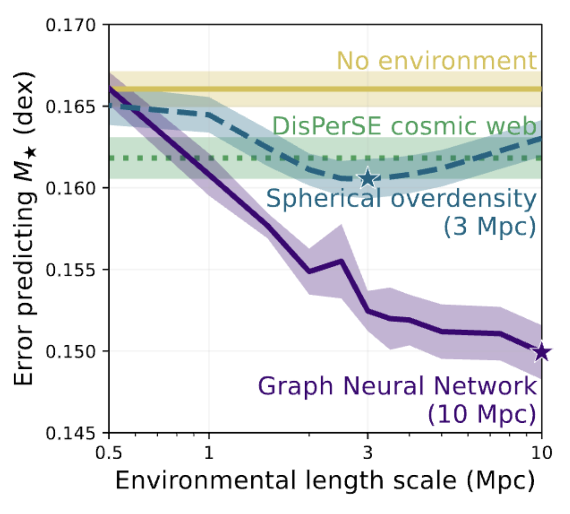
Specifically, we compare machine learning models where no environmental data is provided (yellow), the DisPerSE cosmic web features (green), simple overdensity averaged over a given length scale (blue), and GNNs with graph connectivity on the given length scale (purple). The non-GNN models employed here are explainable boosting machines (EBMs)—decision tree models that are both performant and interpretable. EBMs can receive environmental features on top of the M_subhalo and V_max: think of them as additional columns in a tabular dataset. We can provide EBMs with the collection of DisPerSE features, specify the overdensity on scales ranging from hundreds of kpc to 10 Mpc, or leave out environmental summary statistics altogether.

I want to highlight two main takeaways:

1. Overdensity on 3 Mpc scales is the best simple environmental parameter. Excluding the GNN model, we find that an EBM with spherically averaged overdensity achieves the lowest error for stellar mass predictions. It even outperforms the DisPerSE cosmic web features!
2. GNNs are the undisputed champs. A GNN flexibly processes information on larger scales, and performance continues to improve to the largest distance scales that we test (10 Mpc).

Cosmic graphs are a natural fit for the data, so it’s no surprise that they perform so well. Critically, we construct the graph such that the subhalo position and velocity information is invariant under the E(3) group action; we convert these 6D phase space coordinates into edge features. We’ve also seen hints that this method works in spatial projection, i.e. using 2D spatial coordinates and radial velocities (e.g., see Wu & Jespersen 2023 and Garuda, Wu, Nelson, & Pillepich 2024).

Furthermore, the galaxy–halo connection has different characteristic length scales at different masses. Therefore, the optimality of 3 Mpc overdensity is somewhat specific to our simulation volume and subhalo mass selection. This is another reason to prefer GNNs, which can simultaneously learn the galaxy–halo–environment connection over a huge range of masses and distances.

Graphs adeptly model systems where individual objects are separated by relatively large scales—I mentioned this in the introduction. Meanwhile, much of my research has focused on extracting local information from galaxy systems at the pixel scale by using vision models. We can even combine these two representations by placing a convolutional neural network (CNN) encoder at each node, and letting the GNN process the pixel-level details in tandem with other galaxy parameters (see Larson, Wu, & Jones 2024)!

In summary, cosmic graphs offer a more natural and powerful way to represent the large-scale structure of the Universe than traditional methods. By using GNNs, we can effectively learn the complex relationship between a galaxy’s environment and its properties. In the future, I expect that GNNs will enable new ways to connect simulations to the observable, baryonic Universe.