Graph neural networks in astrophysics

Many physical phenomena exhibit relational inductive biases and can be represented as mathematical graphs. In recent years, graph neural networks (GNNs) have been successfully used to model and learn from astronomical data. This post provides an introductory review to GNNs for astrophysics.

This is the first few sections of an invited review article that’s been sitting around for far too long…

Introduction

Machine learning algorithms have become increasingly popular for analyzing astronomical data sets. In recent years, astronomy’s wealth of data has engendered the development of new and specialized techniques. Many algorithms can learn relationships from catalogued (or tabular) data sets. Vision methods have been adopted across astronomy, e.g., through the use of convolutional neural networks (CNNs) for pixel-level data such as images or data cubes. Time series data sets can be represented using recurrent neural networks or attention-based models. Recently, simulation-based inference and generative models have also become commonplace for solving complex inverse problems and sampling from an implicit likelihood function. I don’t cover these topics here, as other reviews have surveyed the rise of ML applications throughout astronomy, deep learning for galaxy astrophysics, and for cosmology).

Inductive biases of physics problems

Because astronomical data can be structured in various ways, certain model representations are better suited for certain problems. This representational power is tied to the inductive bias of the problem. Multi-Layer Perceptrons (MLPs) or decision tree-based methods operate well on catalog-based data or unordered sets; that is, the permutation of rows or examples does not matter, and the features are treated independently. A CNN is well-suited for data on some kind of pixel or voxel grid; here the features are correlated with each other and have some notion of distance. Graphs are able to represent relationships between entities. See reviews on GNNs, e.g. by Battaglia et al. (2018), Hamilton (2020), Bronstein et al. (2021), and Corso et al. (2024), just to name a few.

What are GNNs?

Graphs are well-suited for representing entities and relationships between them; for example, a “ball and stick” model of a molecule represents atoms as nodes and bonds as edges on a mathematical graph. Another example is a social graph, where people, businesses, and events are different types of nodes, and interactions between these entities (i.e. mutual friends, event attendees, etc.) are edges on the social graph. In addition to the connective structure of the graph, nodes and edges can also be endowed with features. For the molecular graph, node features may comprise positions, atomic weight, electronegativity, and so on.

Because graphs are very general structures, they can offer tremendous flexibility for representing astronomical phenomena. Importantly, they also exhibit relational inductive biases (e.g., Battaglia et al. 2018). Objects that are well-separated from each other are most naturally suited to reside on graph nodes. For example, a galaxy cluster can readily conform to a graph structure: galaxies can be represented as nodes, while interactions between pairs of galaxies (such as gravity, tidal forces, ram pressure, to name a few) can be represented as edges. The circumgalactic medium may be more challenging to represent as a graph, as there exists a continuum of gas densities in multiple phases, each with potentially different lifetimes, making it difficult to draw the line between individual clouds.¹

A graph neural network (GNN) is a machine learning model that can be optimized to learn representations and make predictions on graphs. In this post, I highlight current and future astrophysical applications of GNNs.

Constructing graphs from astronomical data

Before applying a GNN, we’ll need to first construct a graph from our data. The choice of how to define nodes and edges also determines how you might model the data via GNNs. In general, point clouds can be easily represented as nodes on a graph. Objects that are small relative to inter-object separations are natural candidates for nodes, like galaxies, subhalos, stars, or star clusters. The edges, which represent relationships or interactions, can be defined in several ways:

• k-Nearest Neighbors (k-NN): An edge is drawn from a node to its k closest neighbors in physical or feature space. This method ensures that every node has the same number of connections (degree), which can be useful for batching data on a GPU.
• Radius-based: An edge is drawn between all nodes separated by a distance less than a chosen radius r. This is a common choice for representing physical interactions that have a characteristic length scale. Unlike k-NN, this method results in a variable number of connections per node.
• Dynamically: Edges can also be learned dynamically by the model itself, for example, by using an attention mechanism to weight the importance of connections between nodes.

The choice of graph construction method imposes a strong prior on the model, and the best choice will depend the problem.

A primer on mathematical graphs

A graph with \(N\) nodes can be fully described by its adjacency matrix, \(\mathbf{A}\), a square \(N \times N\) matrix that describes how nodes are connected. If an edge connects node \(i\) to node \(j\), then element \(A_{ij}\) has a value of 1; otherwise it is 0. Physical systems are often approximately described by sparse graphs, where the number of edges \(M \ll N(N-1)/2\). This approximation holds if, for example, interactions or correlations between nodes fall off rapidly with distance. A sparse adjacency matrix can also be efficiently represented using a \(2 \times M\) matrix of edge indices. The graph \(\mathcal{G}\) may contain node features \(\mathbf{X}\) and edge features \(\mathbf{E}\), where

Graphs have several characteristics that make them attractive for representing astrophysical concepts. Graph nodes have no preferred ordering, so the operation of a permutation matrix \(\mathbf{P}\) should yield the same graph as before. Critically, models that act on graphs (or sets; Zaheer et al. 2017) can also be made invariant or equivariant to permutations. A permutation-invariant function \(f\) must obey

while a permutation-equivariant function \(F\) must obey

Note that the indices of the edge features are implicitly re-ordered if the permutation operation acts on the adjacency matrix.

Invariant and equivariant models

As discussed above, GNNs are permutation-invariant to the re-ordering of nodes. This invariance reveals a symmetry in the system, as the permutation operator leaves the graph unchanged. Additional symmetries can be imposed on graphs and GNNs, for example, recent works have developed graph models that are invariant or equivariant to rotations and translations in \(3\) or \(N\) dimensions, e.g., (Cohen & Welling 2016, Thomas et al. 2018, Fuchs et al. 2020, Satorras et al. 2021). The subfield of symmetries and representations in machine learning is sometimes called geometric deep learning, and there are far more detailed reviews offered by Bronstein et al. (2021) or Gerkin et al. (2021).

Notwithstanding the far superior review articles mentioned above, I still want to briefly discuss the benefits of leveraging symmetries in astrophysics. While modern ML has demonstrated that effective features and interactions can be learned directly from data, imposing physical symmetries as constraints can vastly reduce the “search space” for this learning task. Perhaps the simplest symmetry is by only using scalar representations. While models that preserve higher-order representations can be more data-efficient (Geiger & Smidt 2022), a simple and powerful way to build invariant models is by contracting all vector or tensor features into scalars (e.g., dot products) at the input layer, as discussed in Villar et al. (2021). Nonetheless, models that allow higher-order internal representations can efficiently learn using fewer data examples.

Other popular models in ML are already exploiting many of these symmetries. Indeed, CNNs, which are commonly used for image data, and transformers, commonly used for text data, can both be considered special cases of GNNs. For example, a convolution layer operates on a graph that is represented on a grid; node features are the pixel values for each color channel, while linear functions over a constant (square) neighborhood represent the convolution operator. CNNs can learn (locally) translation-invariant features, although this invariance is broken if the CNN unravels its feature maps and passes them to a final MLP.

A simple GNN that makes node-level predictions

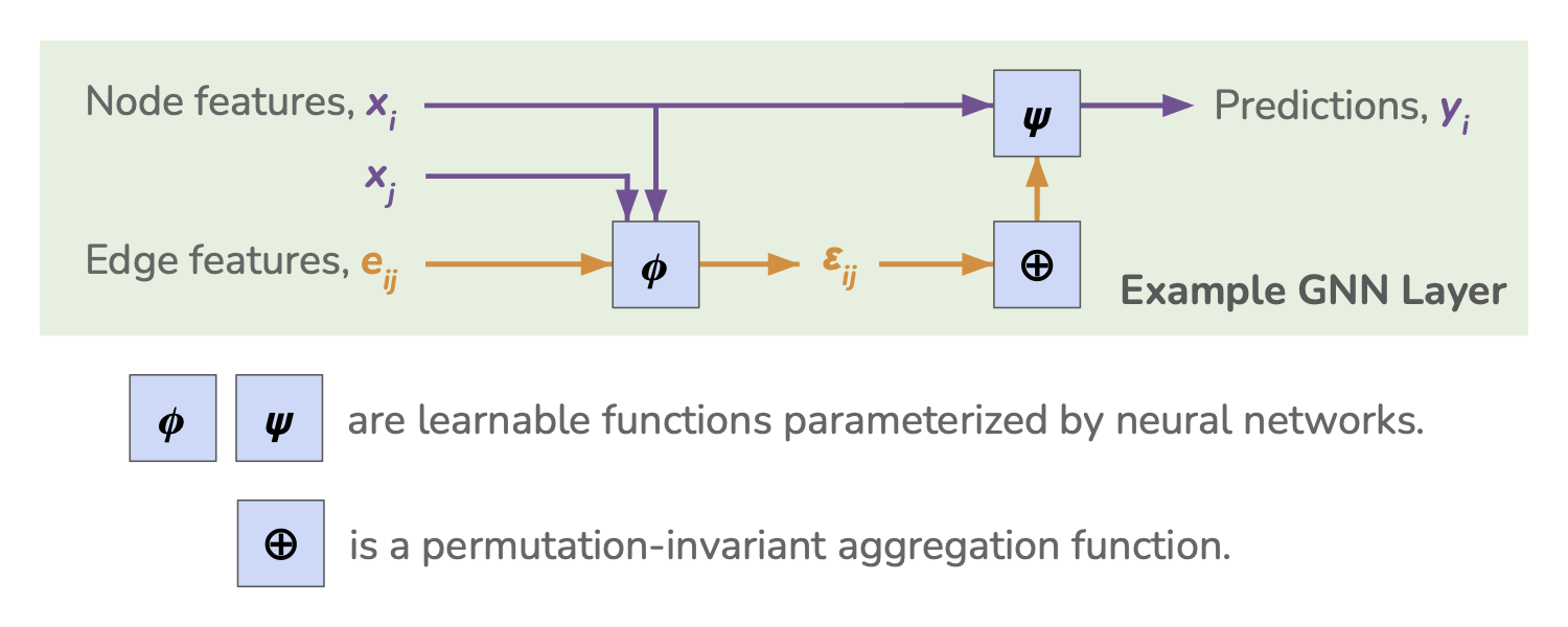Caption: Example of a simple GNN layer that makes node-level predictions. Node features \(x_i\), neighboring node features \(x_j\), and edge features \(e_{ij}\) are fed into a learnable function, \(\phi\), which outputs a hidden edge state \(\varepsilon_{ij}\). All edge states \(\varepsilon_{ij}\) that connect to node \(i\) are aggregated through \(\oplus_j\), a permutation-invariant aggregation function, and the concatenation of its output and the original node features are fed into another learnable function, \(\psi\), which finally outputs predictions at each node \(i\).

Here, we’ll briefly describe the simple GNN illustrated in the above figure. This general structure is often referred to as a message-passing framework. Let’s focus on predictions that will be made on node \(i\). For each neighboring index \(j\), we feed neighboring node features \(x_j\), edge features \(e_{ij}\), and the input node features \(x_i\) into a function \(\phi\) that produces a “message” or edge hidden state \(\varepsilon_{ij}\):

\(\phi\) is a function with shared weights across all \(ij\), and it is parameterized by learnable weights and biases. In practice, \(\phi\) usually takes the form of a MLP with non-linear activations and normalization layers.

An aggregation function \(\oplus_j\) operates on all edge hidden states \(\varepsilon_{ij}\) that connect to node \(i\), i.e., it pools over all neighbors \(j\). Common examples of the aggregation function include sum pooling, mean pooling, max pooling, or even a concatenated list of the above pooling functions. Crucially, the aggregation function must be permutation invariant in order for the GNN to remain permutation invariant.

The function \(\psi\) receives the aggregated messages back at node \(i\), as well as the node’s own features \(x_i\), in order to “update” the node’s state and make predictions: \(y_i = \psi \left (x_i, \oplus_j(\varepsilon_{ij}) \right).\) Similar to \(\phi\), \(\psi\) can be parameterized using a MLP or any other learnable function, so long as the parameters are shared across all training examples.

Although we described just one example of a GNN layer, it serves to illustrate how different kinds of features may interact. Many other alternatives are possible, see e.g., Battaglia et al. 2016, 2018. It is possible to have graph-level features or hidden states that simultaneously act on all node or edge hidden states. Additionally, predictions can be made for the entire graph or on edges rather than on nodes, and likewise, other aggregation patterns are possible.

Prediction tasks on graphs

GNNs are versatile and can be adapted for various prediction tasks depending on the scientific question:

• Node-level tasks: These tasks involve making a prediction for each node in the graph. For example, predicting the stellar mass of a galaxy (node) based on its properties and the properties of its neighbors. The model output is a vector of predictions, one for each node.
• Edge-level tasks: These tasks focus on the relationships between nodes. An example would be predicting whether two dark matter halos will merge, where the prediction is made for each edge connecting two halos.
• Graph-level tasks: These tasks involve making a single prediction for the entire graph. For instance, predicting the total mass (e.g., \(M_{200}\)) of a galaxy cluster (the graph) based on the properties and arrangement of its member galaxies. This usually involves an additional “readout” or “pooling” step that aggregates information from all nodes and edges into a single feature vector before making the final prediction.

Our one-layer GNN described in this section can be extended in two different ways: (i) multiple versions of the learnable functions with unshared weights can be learned in parallel, and (ii) multiple GNN layers can be stacked on top of each other in order to make a deeper network. We now consider \(u = {1, 2, \cdots, U}\) unshared layers, and \(\ell = {1, 2, \cdots, L}\) stacked layers. For convenience, we also rewrite \(x_i\) as \(\xi_i^{(0, \ell)}\), \(x_j\) as \(\xi_j^{(0, \ell)}\), and \(e_{ij}\) as \(\varepsilon_{ij}^{(0, \ell)}\), where the same input features are used for all \(\ell\). (Note that the node and edge input features may have different dimensions than the node and edge hidden states.) With this updated nomenclature, each unshared layer produces a different set of edge states:

which are aggregated and fed into \(\psi^{(u,\ell)}\) to produce multiple node-level outputs:

The extended GNN can have a final learnable function \(\rho\) that makes node-level predictions from the concatenated hidden states:

A connection to multi-headed attention

Another way to say this is by representing \(h_i^{(\ell)}\) as the feature vector of node \(i\) at layer \(\ell\). Assuming that we aggregate all of the unshared layers at each \(\ell\), then \( h_i^{(\ell)} = \oplus_u(\phi^{u,\ell}) \). In that case, the input is \(h_i^{(0)} = x_i\) and a stack of \(L\) layers is then:

Within any single GNN layer, we can learn \(U\) different message functions in parallel — this is just like multi-headed attention (see Veličković et al. 2017)! The outputs of these multiple heads \(\phi^{(1)}, \phi^{(2)}, \cdots, \phi^{(U)}\) can be concatenated (or aggregated) before the final node update: \(\text{final_features}_i = \text{CONCAT}\left[ \bigoplus_j \phi^{(1)}(...), \bigoplus_j \phi^{(2)}(...), \dots \right].\)

Once we’ve extracted this final set of features, we can then pass it through a final learnable function \(\rho\) in order to make predictions.

Summary

Graph neural networks (GNNs) provide a powerful and remarkably intuitive way to model astrophysical systems. By treating objects like galaxies and subhalos as nodes on a graph, we can leverage their physical relationships as edges, making it easier to build models that respect the fundamental symmetries of the problem.

I’ve written this post as a rather general introduction, but real examples can probably paint a clearer picture of how GNNs work. In an upcoming blog post, I’ll highlight some of my own work using these methods to learn the physical connection between galaxies, their subhalos, and their cosmic surroundings. Stay tuned, but if you can’t wait, then you can check out those papers here and here!