Astronomical Super-resolution, Part I: U-Nets

Training a U-Net to enhance images of galaxies.

Prelude

Suppose you want to study a galaxy. Your proposal to target it for follow-up observations has just been accepted—time to tweet it out and let the congratulations flow in! You look in your favorite imaging survey database for a picture of the galaxy so people can see what it looks like (after all, you’ve proposed for spectroscopic observations).

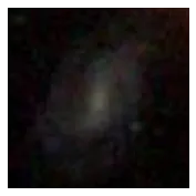
But oh dear, it’s too blurry! You can’t send out a picture like this. People will scroll right past it! Unless… there was some way you could make it look a little better?

Enhance! Enhance! Enhance!

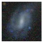
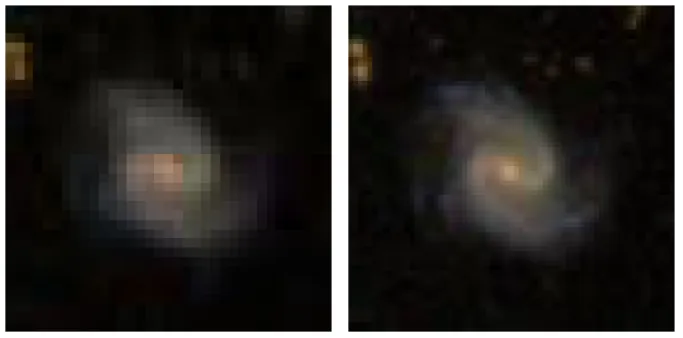
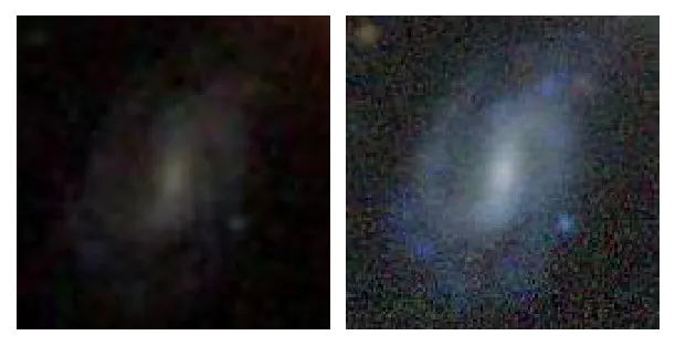
Memes and tired television tropes aside, deep learning might actually be able to get this job done. What if a neural network could enhance this image based on what it knows about the structure of galaxies? In other words, we are trying to perform astronomical image super-resolution, and perhaps get a final result that looks like this:

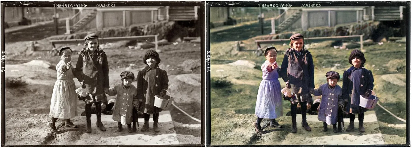
Is it possible? The answer is… maybe. It really depends on your data set and use case. But we’ve been surprised by the power of deep learning before: grainy black and white photographs from the early 1900s can be colorized and modernized! In this case, deep learning can recolor and restore old photographs, because people, grass, and houses from back then still kind of look like people, grass, and houses today. Another reason for deep learning’s success is that we are able to create excellent training data sets, since it is simple to convert a color image to monochrome or add noise.

Super-resolution as a toy problem

Let’s see if we can artificially add noise or blur out astronomical images in a realistic manner. I’m calling this a toy problem because we’re generating our own corruptions to the data. I will use the SDSS data set (Galaxy10) mentioned in my last blog post. We can load the images from the hdf5 file and ignore their morphological classification labels.

Next, we want to make crappy versions of the original images. We can corrupt the images in two ways: (a) down-sizing the images by a factor of two (i.e., from 69×69 → 35×35), and (b) adding Poisson-distributed noise. These transformations can be implemented using skimage.transform.downscale_local_mean() and skimage.util.random_noise() from the scikit-image library.

Training a U-Net generator

To reconstruct the corrupted galaxy image, we will need a convolutional neural network (CNN) model that can not only ingest images, but also output them. Last time we used a variational autoencoder to do something like this. However, we can do better this time with a U-Net!

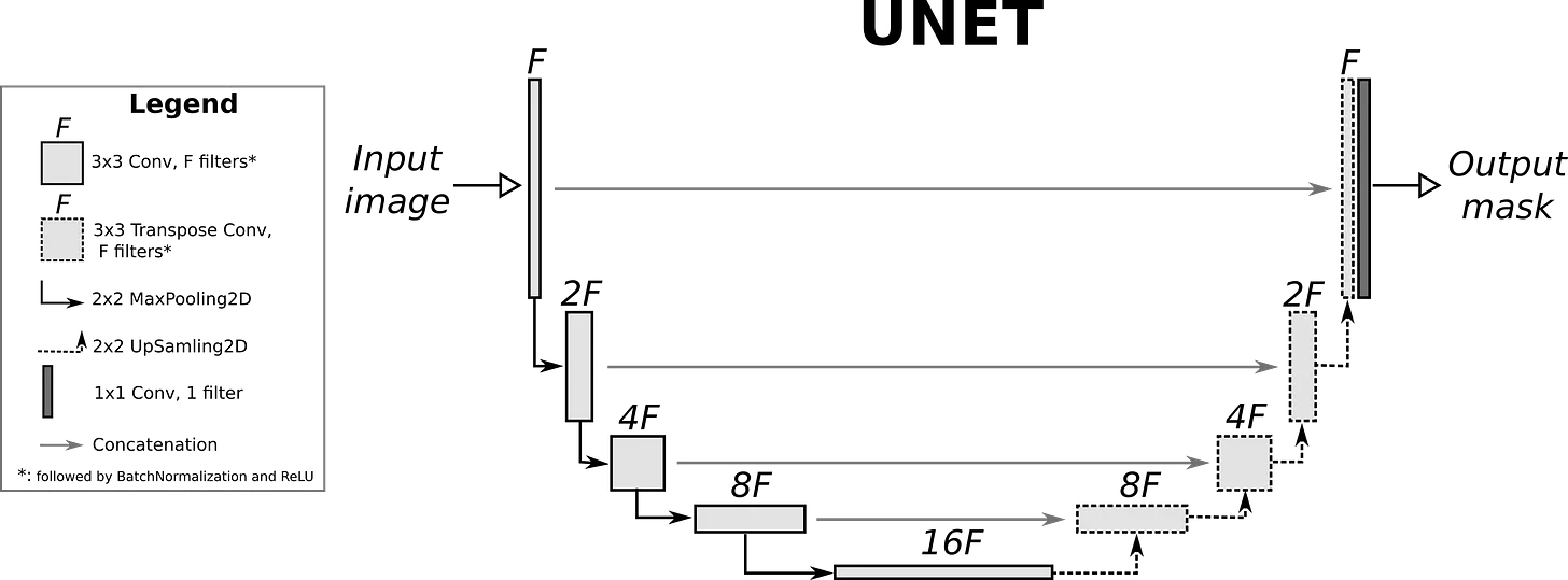
In addition to a encoder plus decoder components (known as the downsampling and upsampling paths on the left and right, respectively), U-Nets have skip connections that concatenate activations from the downsampling layers to the analogous upsampling layers. The downsampling path looks a lot like a CNN, and indeed we can create a U-Net model based on a CNN architecture.

To get this working, I consulted the incredible “Walk with Fastai” resource by Zach Mueller, which covers a large number of applications with the high-level Fastai library (built atop Pytorch). Both Zach’s guide and the Fast.ai docs give some guidance for using fastai.vision.learner.unet_learner(), which creates a complementary upsampling path given a CNN downsampling model.

We can either train the U-Net from scratch (random initialization), or we can take advantage of transfer learning. For the latter case, we would require a pre-trained CNN model for the downsampling path. Even though astronomical images are quite dissimilar to terrestrial images such as the ones in the ImageNet data set, I’ve previously shown that a model pre-trained on ImageNet work extremely well when fine tuned on smaller astronomical data sets. This is probably because the first few layers of CNNs nearly always identify features like edges and Gabor filters, so they can be generalized to quite different image recognition tasks.

Once we have collated our data, constructed our U-Net, and defined a loss function (mean squared error), we are ready to train the model!

A very modest enhancement

We can efficiently fine-tune the network by first training the upsampling path while freezing the resnet-18 part of the model, and then training the entire U-Net for a few more epochs. Let’s look at the results:

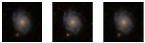
Here we see a low-resolution corrupted image (left), the original image (center), and our U-Net reconstruction (right). The enhancement doesn’t seem all that impressive — certainly nothing like the portrayal of such algorithms in CSI.

In particular, the fine details have not been recovered. Spiral arms that have been blurred out by our artificial corruption remain blurry. However, if you look closely, you can see that JPG compression artifacts (the block patterns, which are present in both the original and the corrupted images) have been mitigated in the U-Net enhanced image.

Super-resolution as a realistic astronomical problem

We’ve found that our toy problem didn’t work so well. The final results appear to be limited by Nyquist sampling, and by our rather small data set. Our toy problem is still too hard: a factor of two reduction in image resolution destroys too much information. [Perhaps a deep neural network ](can learn how to paint in information below the sampling or deconvolution limit. But we don’t have enough data to train a U-Net generator to figure out what kinds of image patterns should appear below the resolution limit.

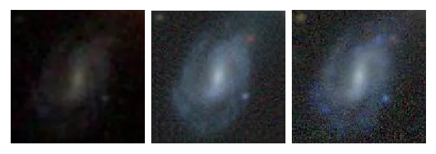
Let’s now consider another problem. Suppose we have a shallower, lower-resolution set of images from the Sloan Digital Sky Survey (SDSS), but we wish we had deeper, higher resolution images from the Dark Energy Camera Legacy Survey (DECaLS). In fact, this is exactly the use case that we presented at the top of this post!

SDSS images have pixel sizes of 0.396 arcsec while DECaLS images have 0.262 arcsec pixels, so in some sense we are still doing “super-resolution.” Another challenge is for the U-Net to learn how to boost the signal-to-noise ratio. Features that are on the cusp of non-detection in SDSS are clearly detected in DECaLS. (DECaLS images also look bluer in SDSS imaging due to different telescope filters being used in the false-color RGB images.)

Our model should only be used for typical SDSS galaxies. As we have discussed above, we cannot extrapolate to other data sets or galaxy samples that aren’t representative of our training data, e.g., oddball galaxies with bizarre properties or extremely distant galaxies that can only be detected by other telescopes.

The magic of U-Nets

We can set up our problem as before, now with minimal pre-processing. All we have to do is to obtain galaxy images from both SDSS and DECaLS and ensure that they have the same angular sizes. I’ve elected to use a large sample of 142,000 galaxies studied in one of my previous papers so that we can train our U-Net from scratch (and for longer). This time, the U-Net seems to perform quite well!

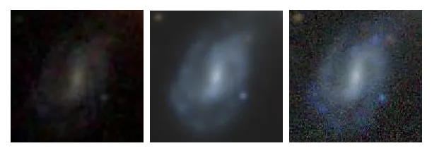
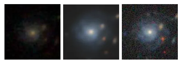
Our model is able to recover some of the faint, barely detected features in SDSS imaging. In the examples below, we can see that the U-Net has unearthed spiral arms and lower-surface brightness galaxy disks. Sometimes it is also able to amplify point sources that aren’t even related to the main galaxy.

However, we can also see some obvious errors. The noise profiles in the generated images is completely wrong; they’re too smooth! In fact, all of the generated images look like they’ve been smoothed out.

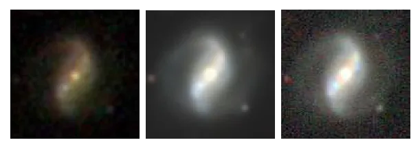
In order to produce more realistic DECaLS images, we can also train a GAN. Compare the previous images with their corresponding GAN outputs (center column) below:

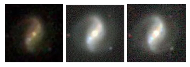
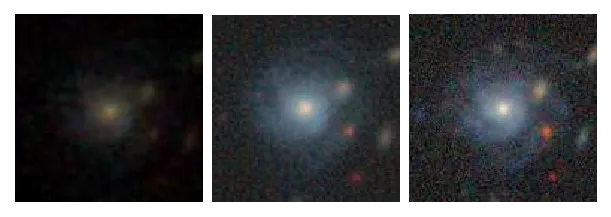
Looks much more realistic! If you want to learn more, please tune in to Part II of this blog post series, where I will cover GANs in a bit more detail.

Until next time!

You can find some of the code for this post in this Github Gist. Credit also goes to the Fast.ai 2019 course (Jeremy Howard) and Walk with Fastai (Zach Mueller).

This post was migrated from Substack to my blog on 2025-04-23