Astronomical Super-resolution, Part II: GANs

Generative adversarial networks are magical… when they work.

Prelude

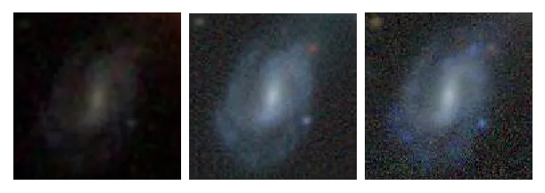
Let’s pick up where we left off in the previous post. Wait, has it been a year already? Okay, we really need to review what we did last time. We’ve got a faint image of this galaxy from the Sloan Digital Sky Survey (SDSS; left), but we wish we had the corresponding high-fidelity version from the Legacy Survey (DECaLS, right).

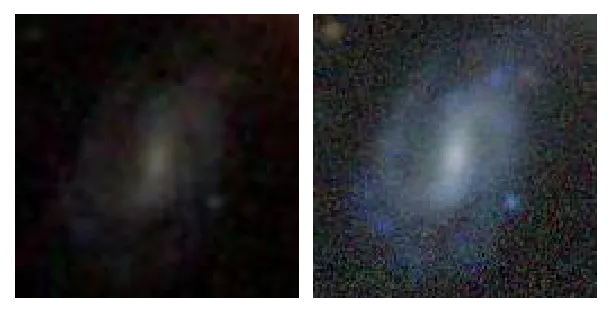
Somehow, we want to turn the left-side image into the right-side one. Last time we used a U-net, which is a convolutional architecture that takes images as inputs and predicts images as outputs. The technical details can be found in this Jupyter notebook.

We will use a sample of 142,000 galaxies with detectable star formation rates and metallicity measurements, which is larger than the data set we used last time. However, this sample isn’t representative of all galaxies in the Universe; many galaxies are no longer forming new stars, and we might expect our deep learning algorithm (once trained) to give unexpected results on them. Assuming that we don’t fall prey to this “domain shift” problem, let’s proceed to discuss some more generative algorithms.

Autoencoders and U-Nets: a review

Previously, we investigated Autoencoders and U-Nets, which are convolutional neural networks (CNNs) that can downsample an image and then upsample it again. Autoencoders will reconstruct the same image that was input (hence the name autoencoder), whereas U-Nets learn to construct a different image from the input. In order to increase resolution (and remove aliasing artifacts), the upsampling path will need to contain transposed convolutions plus interpolation or PixelShuffle with ICNR initialization. The result is that each layer’s activations will decrease like 224×224 → 112×112 → 56×56 → … in the downsampling path, and then increase again like … → 56×56 → 112×112 → 224×224 in the upsampling path.

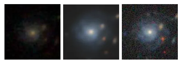
As we saw in Part I, U-Nets can successfully increase image brightness/contrast and enhance barely detected objects — even picking them out from the background noise. However, the main problem is that U-Net reconstructions are too blurry. For example, the predicted image above (center) does not really resolve the galaxy’s spiral arms. This could be due to the fact that the SDSS input image completely fails to detect any spiral arms, so there is nothing to enhance! Despite such limitations, it might be possible for a deep learning generative model to figure out whether a dim galaxy image should contain spiral arms simply from the context of the rest of the image.

We will need a powerful model to accomplish such a task. And this model — really the interplay between two neural networks — is called a generative adversarial network (GAN; introduced by Goodfellow et al. 2014).

A tip-of-the-iceberg overview of GANs

A GAN consists of two neural networks: a generator and a critic. We can use a U-Net as the generator, as we did before. The critic tries to differentiate between generator predictions (e.g., enhanced and super-resolved SDSS images) and the targets (e.g., the DECaLS images), perhaps by way of a cross-entropy loss, or the Wasserstein metric (aka Earth-Mover distance), or a loss conditioned on galaxy metadata such as morphological labels, or something else. Thus, the critic competes directly against the generator (hence adversarial network); they can be thought of as two players in a zero-sum game. If the generator starts to produce more plausible outputs, then the critic will also need to wise up!

All sorts of interesting game theory phenomena can emerge from training these two networks. One way to gain insight into the dynamics of optimizing GANs is by visualizing the game vector field instead of either model’s loss landscape.

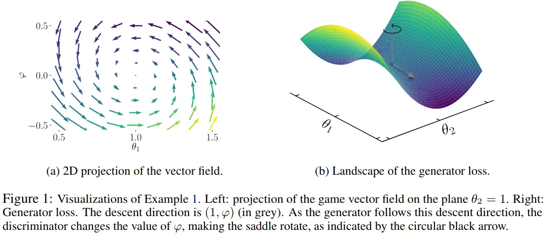
The two-player game causes the generator (U-Net) loss function to rotate, which makes optimization difficult (see paper here). Even worse, the rotation isn’t even about a local minimum in the loss surface — in the example above the optimization will run circles around a saddle point!

In order to get around some of these optimization challenges, various methods such as WGAN have been proposed (see this post for details on some of mathematics behind GAN and WGAN models). The W in WGAN stands for the Wasserstein metric, which provides a way to measure differences between the generated/enhanced images and the true high-fidelity images. Using the Wasserstein metric in the loss function helps improve stability and expressivity when training GANs. However, we won’t go there today; we will instead implement a simple BCE loss function for the critic (binary cross-entropy loss), which can be susceptible to mode collapse or other issues.

Once the generator’s loss plateaus, or after a set number of training epochs, we can save a bunch of the generated image outputs. This can be thought of as a “pre-training” step for the generator. Then, we can begin pre-training the critic for a few epochs. We’ve assembled the GAN!

After the generator and critic have both been pretrained, we should set up a rhythm of switching between training one or the other. We implement a “switcher callback” that automatically switches from training one to the other depending on whether the critic or generator becomes too dominant. We also need to tweak the hyperparameters for the two networks; in particular, the critic usually needs a higher learning rate than the generator in order for the GAN to operate well.

Since the loss rises and dips cyclically, it can be hard to gauge when to stop. Thus, it’s useful to frequently visualize the low-resolution inputs, high-fidelity ground truths, and GAN-enhanced images. Below you can see some results:

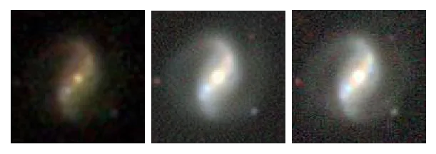
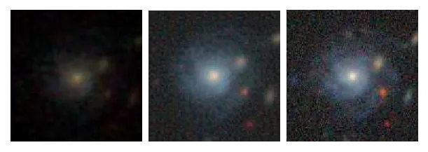
These look better than our smudge-y predictions purely from a U-Net!

Future improvements?

The GAN loss functions are extremely important. If we simply use a mean squared error loss, the generator will often compromise on a “safe solution” — usually one that is fairly blurry and muted in color. Terms like perceptual loss (aka feature loss), or “stability loss” can be very useful. We might also rely on the WGAN method described above. Finally, we could also add self-attention layers to the GANs and progressively increase the resolution in multiple stages, as is done in this repository.

There are plenty of other alternatives to this kind of generative work. One great example in astronomy is a simulation-based inference approach (i.e., using deep neural nets for inverse problems), presented by Francois Lanusse during a recent CMU Quarks2Cosmos hackathon. You can find the guided data challenge here, with notebooks on forward modelling, generative modeling with normalizing flows, and variational inference.

The associated Jupyter notebook can be viewed on Github or run on Colab. Many thanks to Zach Mueller for his Walk with Fastai tutorials.

This post was migrated from Substack to my blog on 2025-04-23