What do galaxies look like? Learning from variational autoencoders

Exploring the latent space of galaxy images with autoencoders.

Prelude

How much information do we actually use from astronomical imaging? I’ve always wondered about this as I gaze at wide-field survey imaging data. After all, galaxies are complex collections of stars, gas, and dust, but for convenience, astronomers often represent them using just a few numbers that describe their colors, shapes, and sizes. Seems a bit unfair, right?

It’s for this reason that I got interested in using machine learning to utilize all the information that’s available in astronomical images—down to the pixel scale. (You can read about my first foray into deep learning in a previous post). As machine learning methods continue to grow more popular in the astronomical research community, it seems more and more apparent that we should be using convolutional neural networks (CNNs) or other computer vision techniques to process galaxies’ morphological information. These models are flexible enough to make sense of diverse galaxy appearances, and connect them to the physics of galaxy evolution.

Up until now, however, I’ve mostly used CNNs to make predictions—a form of supervised machine learning. There are other unsupervised or semi-supervised methods, which generally try to teach a model to learn about the underlying structure of the data. For example, we might expect that a model should be able to figure out that the same galaxy can be positioned at different angles or inclinations, and that it could supply a few variables to encode the orientation of the system. Unsupervised machine learning models can figure out these kinds of patterns without explicitly being taught the position angle or inclination.

So I set out to experiment a bit with some unsupervised models (specifically autoencoders—more on that later). But first, I needed a good data set!

Stumbling across a neat data set

I had the pleasure of attending the NeurIPS 2020 conference and presenting some recent work during one of the workshops three weeks ago. During one the talk/tutorial sessions, I found out about a neat little dataset called Galaxy10, which is a collection of 21,000 galaxy images and their morphological classifications from GalaxyZoo (which, by the way, is a citizen science project). Galaxy10 is meant to be analogous to the well-known Cifar10 data set frequently used in machine learning.

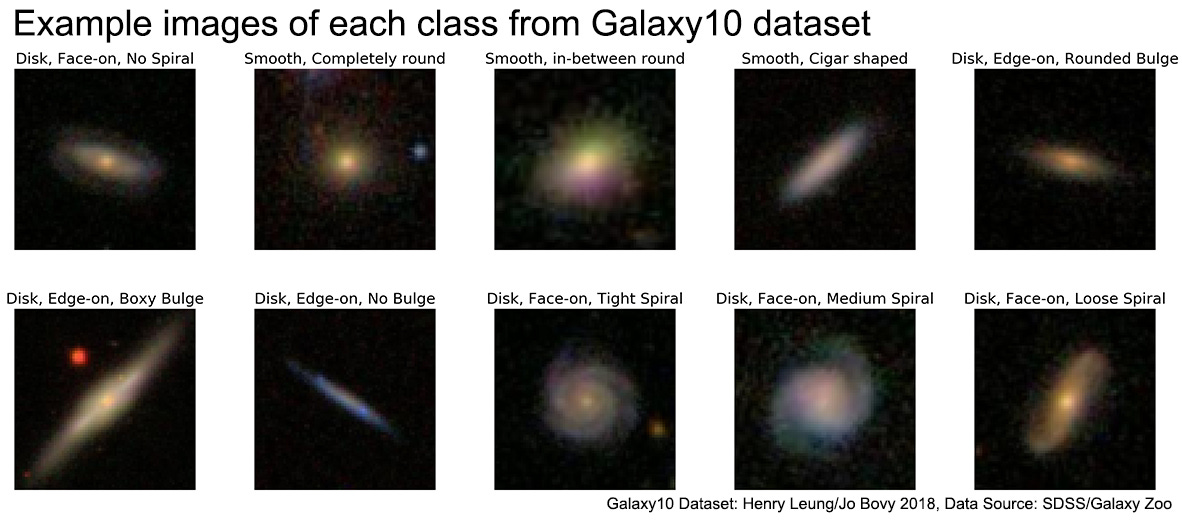
Since these images are extremely morphologically diverse, and the data set seemed to be free from corrupted images and other artifacts, I decided to train an autoencoder to reconstruct these images.

(If you want to jump straight to the code, take a look at my Github repository.)

What is an autoencoder?

In short, an autoencoder is a type of neural network that takes some input, encodes it using a small amount of information (i.e., a few latent variables), and then decodes it in order to recreate the original information. For example, we might take a galaxy image that has 3 channels and 69×69 pixels (for a total of 14,283 pieces of information), and then pass it through several convolution layers so that it can be represented with only 50 neurons, and then pass it through some transposed convolutions in order to recover the original 3×69×69 pixel image. It is considered an unsupervised learning model because the training input and target are the same image—no other labels are needed!

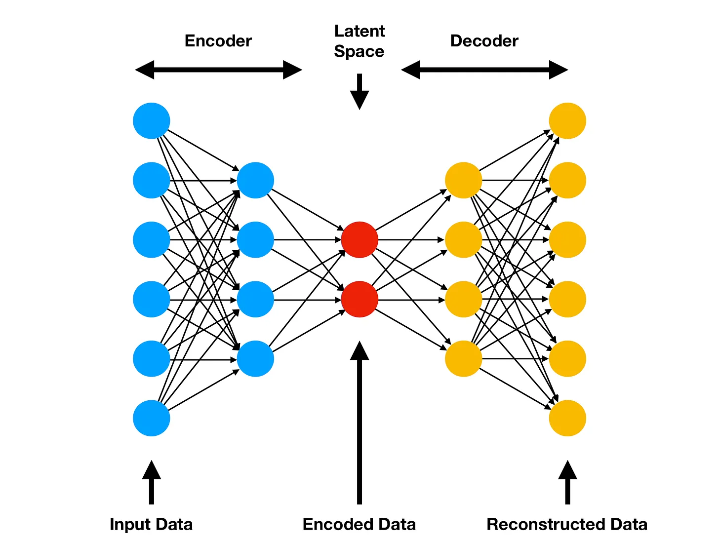
An autoencoder is essentially a compression algorithm facilitated by neural networks: the encoder and decoder are learned via data examples and gradient descent/backpropagation. Another way to think about it is a non-linear (and non-orthogonal) version of principal components analysis.

I decided to use a variational autoencoder (VAE), which probabilistically reconstructs the inputs by sampling from the latent space. That is, the model learns a set of latent variable means and variances, from which it can construct a multivariate normal distribution. It will then select points near the encoded latent variable and compare decoded outputs to the original inputs; this ensures that the latent space is smoothly varying. There is a lot more to variational inference than what I’ve written here, so please feel free to check out other resources on the matter (e.g., this blog post). While training VAEs, we often find that the latent space contains interpretable information about the structure of the inputs.

Exploring VAE loss functions

I experimented with a few different terms in the VAE loss function: evidence lower bound (ELBO), maximum mean discrepancy (MMD), perceptual loss, and class-aware cross-entropy loss.

All loss functions should penalize the pixel reconstruction error, so I imposed a mean squared error (MSE) penalty for differences between the input and output pixel values. In essence, the reconstruction error makes sure that every pixel in the output image actually looks like the corresponding one in the input image. ELBO comprises the MSE and a Kullback–Leibler (KL) divergence term. The KL divergence measures the dissimilarity between the multivariate normal distribution (a simplifying assumption that we made as part of our VAE) and the true underlying probability distribution of a latent variable given some input.

However, optimizing a VAE using ELBO tends to blur out information that isn’t well-represented in the input examples; this is a common problem with vanilla VAE models. See this explanation, which does a great job of explaining why we need additional loss terms to rectify this problem. MMD is one such term that penalizes the level of dissimilarity between the moments of the learned and underlying distributions. Other loss terms like perceptual loss or class-aware loss may help enforce certain inductive biases that make reconstructions more expressive or informative. However, based on my limited experience, the MMD term used in information-maximizing VAEs (InfoVAEs) is sufficient to get excellent results.

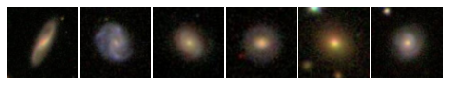
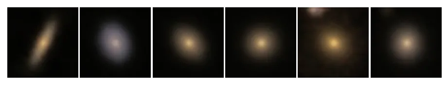
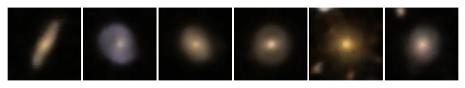
In this comparison, I show six input images (top), reconstructions from a VAE trained with ELBO for 50 epochs (middle), and reconstructions from a VAE trained with MMD for 50 epochs (bottom). We can see that the MMD term enables reconstructions with more detailed features, such as spiral arms, non-axisymmetric light distributions, and multiple sources. In other words, the MMD-VAE is able to encode galaxy images with higher fidelity than the ELBO-VAE.

Of course, the level of detail can still be improved. We have only used a small subsample of galaxies from the Sloan Digital Sky Survey, and of course we might get nicer results if we used a survey telescope with higher-resolution imaging. Another way to produce a higher level of reconstruction detail is to use generative adversarial networks (GANs) or flow-based generative models. But let’s save those for another post.

Using the VAE decoder as a generator

Once we have trained a VAE, we can now interpolate across examples in the latent space and reconstruct outputs from these vectors. What do they mean?

Making neural networks hallucinate is always profitable. (See, e.g., awesome blog post by Jaan Altosaar and sweet demos from OpenAI, and distill.pub.) So I decided to take a journey through the imaging latent space, decode the outputs, and animate them in GIF format:

Pretty neat huh? It’s quite interesting to see how ELBO encourages the model to learn broad-brush features, which are mostly those that can be easily represented by classical morphological parameters such as concentration, ellipticity, etc. The MMD variant learns way more complicated features!

We can also just directly decode each vector as well in order to see the image feature that correlates with each latent variable. Here I’m stepping through the latent space of the ELBO-VAE. (Note that Nσ refers to the number of standard deviations from the mean in each dimension of the latent space).

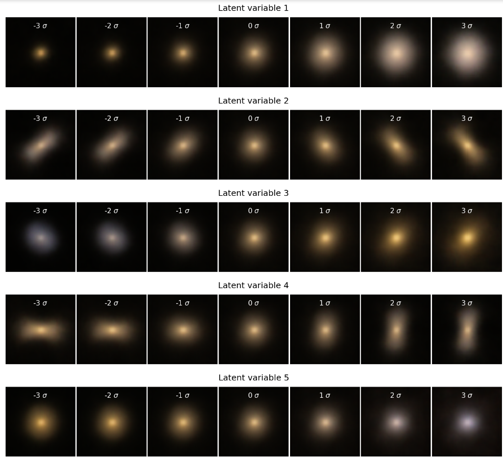
Imagine all this with incredibly high-resolution imaging! Now I really can’t wait for the Nancy Grace Roman Space Telescope to launch.

All of the code to make the figures in this notebook can be found in my Github repository. Questions? Violent objections? Send them my way on Twitter or email. Or subscribe to see my next post!

This post was migrated from Substack to my blog on 2025-04-23